- A. (ICLR 2017) Towards Principled Methods for Training Generative Adversarial Networks
- B. (ICML 2017) Wasserstein generative adversarial networks
- 参考文献
这篇笔记包含了 Martin Arjovsky 的两篇分析原始 GAN 中存在的问题的文章1 2. Martin Arjovsky 来自于纽约大学柯朗数学研究所(Courant Institure of Mathematical Science). 其导师是就职于 FAIR 的 Leon Bottou.

图 1. 纽约大学柯朗数学研究所
A. (ICLR 2017) Towards Principled Methods for Training Generative Adversarial Networks
本文提出了 GAN 训练中存在的四个问题: • 为什么随着判别器越来越好, 生成器变得越来越差? 无论是用原始损失(Jensen-Shannon divergence, JSD)还是新的损失函数? • 为什么 GAN 的训练非常不稳定? • 新的损失函数是否是和 JSD 相似的 divergence?, 如果是, 他们有什么共同点? • 是否有办法避免这些问题?
GAN的总目标函数是:
\[\min_G\max_D V(D,G)=\mathbb{E}_{\mathbf{x}\sim p_{\text{data}}(\mathbf{x})}[\log D(\mathbf{x})]+\mathbb{E}_{\mathbf{z}\sim p_{\mathbf{z}}(\mathbf{z})}[\log(1-D(G(\mathbf{x})))].\]训练判别器:
\[\max_{D} \mathbb{E}_{\mathbf{x}\sim p_{\text{data}}(\mathbf{x})}[\log D(\mathbf{x})]+\mathbb{E}_{\mathbf{z}\sim p_{\text{data}}(\mathbf{z})}[\log (1-D(G(\mathbf{z})))]\]训练生成器:
\[\min_{G} \mathbb{E}_{\mathbf{x}\sim p_{\text{data}}(\mathbf{x})}[\log (1-D(G(\mathbf{z})))]\]1. 不稳定性的来源
1.1 完美判别器
If two distributions \(\mathbb{P}_r\) and \(\mathbb{P}_g\) have support contained on two disjoint compact subsets \(\mathcal{M}\) and \(\mathcal{P}\) respectively, then there is a smooth optimal discrimator \(D^*: \mathcal{X} \rightarrow [0,1]\) that has accuracy 1 and \(\nabla_xD^*(x)=0\) for all \(x\in \mathcal{M}\cup\mathcal{P}.\)
定理1告诉我们如果两个分布的支撑分别包含在两个不相交的集合中, 那么存在一个最优的判别器使得任意位置的梯度都是0.
Let \(\mathbb{P}_r\) and \(\mathbb{P}_g\) be two distributions whose support lies in two manifolds \(\mathcal{M}\) and \(\mathcal{P}\) that don’t have full dimension and don’t perfectly align. We further assume that \(\mathbb{P}_r\) and \(\mathbb{P}_g\) are continuous in their respective manifolds. Then, \(\begin{align}\nonumber JSD(\mathbb{P}_r\Vert\mathbb{P}_g) &= \log2 \\ \nonumber KL(\mathbb{P}_r\Vert\mathbb{P}_g) &= +\infty \\ \nonumber KL(\mathbb{P}_g\Vert\mathbb{P}_r) &= +\infty \\ \end{align}\nonumber\)
定理2告诉我们如果两个分布的支撑分别包含在两个不 perfectly align 且是绝对的子流形上, 并且两个分布在各自的流形上都连续, 那么存在最优的判别器使其在两个流形上的任意点的准确率都是1, 在任意点的领域内都连续, 且导数为0.
这个定理告诉我们用divergence来测试两个分布的相似度的话, 我们可以得到一个完美的判别器, 即判别器对 Pr 和 Pg 上的样本都能够完美判别(恒为1或0), 所以无法产生梯度, 进而无法训练模型参数.
1.2 结论, 损失函数存在的问题
Let \(g_{\theta}:\mathcal{Z}\rightarrow\mathcal{X}\) be a differentiable function that induces a distribution \(\mathbb{P}_r\). Let \(\mathbb{P}_g\) be the real data distribution. Let \(D\) be a differentiable discriminator. If the conditions of Theorems 1 or 2 and satisfied, \(D-D^*<\epsilon\), and \(\mathbb{E}_{z\sim p(z)}[\Vert J_{\theta}g_{\theta}(z)\Vert_2^2]\leq M\), then \(\Vert \nabla_{\theta}\mathbb{E}_{z\sim p(z)}[\log(1-D(g_{\theta}(z)))]\Vert_2<M\frac{\epsilon}{1-\epsilon}\)
Under the same assumptions of Theorem 4 \(\lim_{\Vert D-D^*\Vert\rightarrow0}\nabla_{\theta}\mathbb{E}_{z\sim p(z)}[\log(1-D(g_{\theta}(z)))]=0\)
从定理4可以得到上面的推论: 随着判别器越来越好, 生成器的梯度在逐渐消失. 实验结果也验证了这一点.
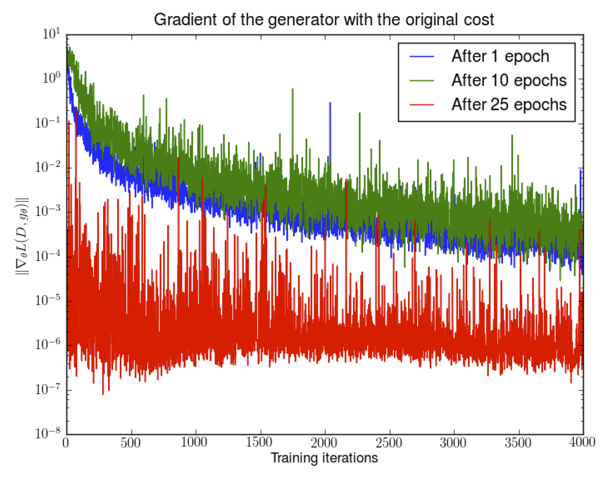
图 2. 随着判别器越来越好, 生成器的梯度在逐渐消失
后来人们采用 -logD 梯度来进行优化:
Let \(\mathbb{P}_r\) and \(\mathbb{P}_g\) be two continuous distributions, with densities \(P_r\) and \(P_{g_{\theta}}\) respectively. Let \(D^*=\frac{P_r}{P_{g_{\theta_0}}+p_r}\) be the optimal discriminator, fixed for a value \(\theta_0\). Therefore, \(\mathbb{E}_{z\sim p(z)}[-\nabla_{\theta}\log D^*(g_{\theta}(z))\vert_{\theta=\theta_0}]=\nabla_{\theta}[KL(\mathbb{P}_{g_{\theta}}\Vert\mathbb{P}_r)-2JSD(\mathbb{P}_{g_{\theta}}\Vert\mathbb{P}_r)]\vert_{\theta=\theta_0}\)
这样, 生成器的损失函数可以推出定理5的结果. 从式中可以看出,
- 极小化生成器损失会使得两个分布的 JSD 距离变大, 这不符合我们优化的目标
- 极小化 KL 散度. 我们知道 KL 散度在生成错误样本时 cost 非常大, 而在发生 mode dropping 的时候 cost 非常小.
接下来讨论一个最优判别器加上噪声后形成的判别器的不稳定性.
Let \(g_{\theta}:\mathcal{Z}\rightarrow\mathcal{X}\) be a differentiable function that induces a distribution \(\mathbb{P}_g\). Let \(\mathbb{P}_r\) be the real data distribution, with either conditions of Theorems 1 or 2 satisfied. Let \(D\) be a discriminator such that \(D^* - D=\epsilon\) is a centered Gaussian process indexed by \(x\) and independent for every \(x\) (polularly known as white noise) and \(\nabla_xD^*-\nabla_xD=r\) another independent centered Gaussian process indexed by \(x\) and independent for every \(x\). Then, each coordinate of \(\mathbb{E}_{z\sim p(z)}[-\nabla_{\theta}\log D(g_{\theta}(z))]\) is a centered Cauchy distribution with infinite expectation and variance.
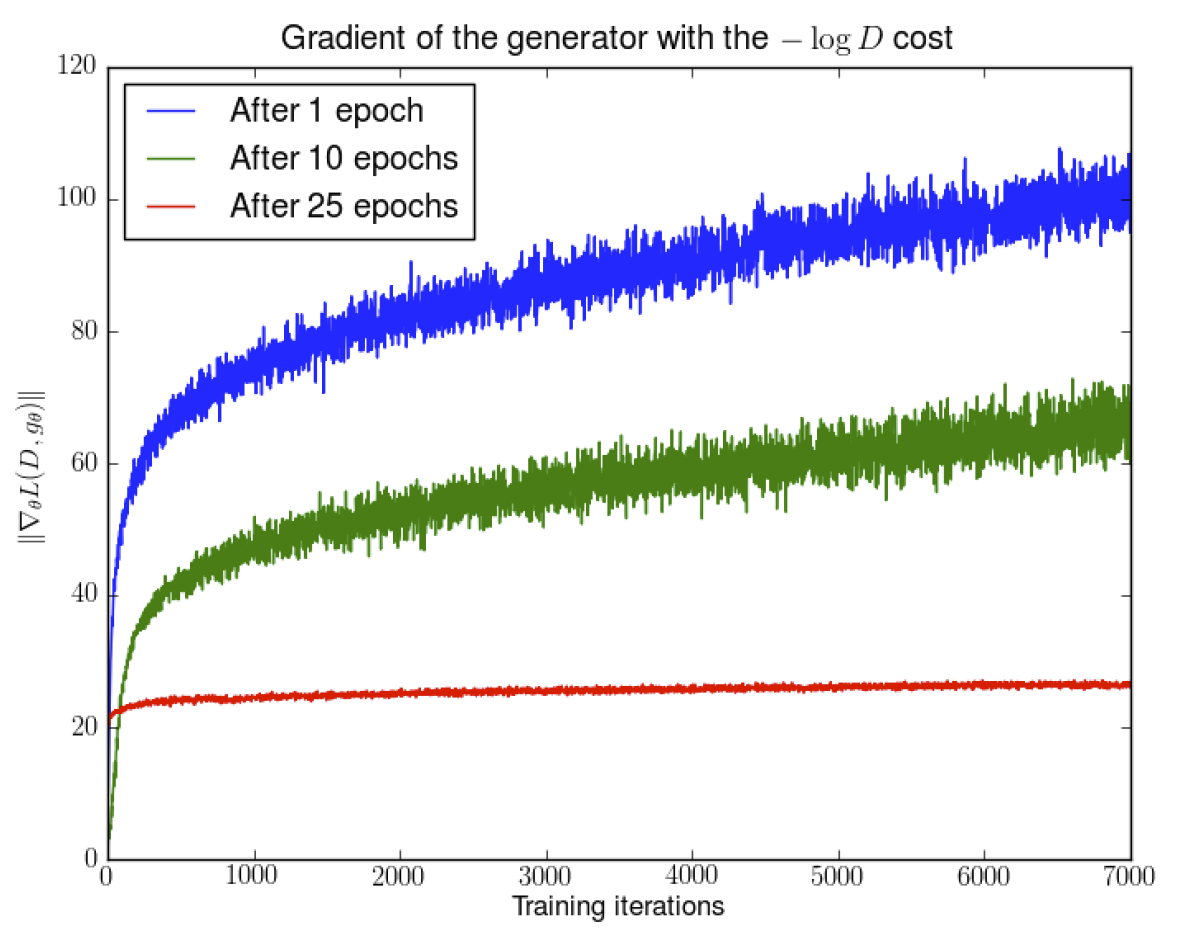
图 3. 在判别器接近最优时, 其梯度的情况
上图显示了在判别器接近最优时, 其梯度的情况, 可以发现梯度越来越大, 并且方差也越来越大.
2. 软指标和分布
那么如何解决生成器梯度消失和判别器不稳定的问题呢?
首先, 为了破坏前述定理的条件, 即判别器输入 Pr 和 Pg 分布的不相交, 我们可以在判别器的输入上加一个空间中连续的噪声, 这样可以平滑化两个输入分布的概率密度.
If \(X\) has distribution \(\mathbb{P}_X\) with support on \(\mathcal{M}\) and \(\epsilon\) is an absolutely continuous distribution with density \(P_{\epsilon}\), then \(\mathbb{P}_{X+\epsilon}\) is absolutely continuous with density \(\begin{align} P_{X+\epsilon}(x) &=\mathbb{E}_{y\sim \mathbb{P}_X}[P_{\epsilon}(x-y)] \\ &=\int_{\mathcal{M}}P_{\epsilon}(x-y) d\mathbb{P}_X(y) \end{align}\)
这个定理告诉我们, 加了连续噪声的分布反比于Px的支撑中点的平均距离. 而噪声分布的选择也影响着距离的表示方式, 现在最优的判别器变成了 \(D^*(x)=\frac{P_{r+\epsilon}(x)}{P_{r+\epsilon}(x)+P_{g+\epsilon}(x)}\) 接下来我们看生成器的梯度:
Let \(\mathbb{P}_r\) and \(\mathbb{P}_g\) be two distributions with support on \(\mathcal{M}\) and \(\mathcal{P}\) respectively, with \(\epsilon\sim\mathcal{N}(0, \sigma^2I)\). Then, the gradient passed to the generator has the form
\(\begin{align}
\mathbb{E}_{z\sim p(z)} &[\nabla_{\theta}\log(1-D^*(g_{\theta}(z)))] \\
&=\mathbb{E}_{z\sim p(z)}[a(z)\int_{\mathcal{M}}P_{\epsilon}(g_{\theta}(z)-y)\nabla_{\theta}\Vert g_{\theta}(z)-y\Vert^2 \mbox{d}\mathbb{P}_r(y)] \\
&=-b(z)\int_{\mathcal{P}}P_{\epsilon}(g_{\theta}(z)-y)\nabla_{\theta}\Vert g_{\theta}(z)-y\Vert^2 \mbox{d}\mathbb{P}_g(y)]
\end{align}\)
where \(a(z)\) and \(b(z)\) are positive functions. Furthermore, \(b>a\) if and only if \(P_{r+\epsilon}>P_{g+\epsilon}\), and \(b > a\) if and only if \(P_{r+\epsilon}<P_{g+\epsilon}\) .
这个定理证明了我们此时产生的样本 趋向数据的流形, 同时是样本和数据的概率以及距离加权的结果. 进一步, 第二项驱使我们生成的样本远离 \(P_g\) 分布上的点(因为是假的样本), 这一点很重要. 因为当 \(P_g > P_r\) 的时候, 有 \(b > a\), 此时第二项就有更强的动力去把生成的样本点推离假的样本.
实际上加了噪声多少都会影响模型最终学习到的效果, 因此我们希望控制噪声的幅度要尽可能小. 但是作者指出,
随着加的噪声逐渐减小, 就越来越接近 , 最终导致 会 max out.
这里我的理解是, JSD 距离不能随着 \(\epsilon\) 方差的减小而减小. 所以作者提出使用的 Earth Mover’s Distance (也叫 Wasserstein 距离)可以避免这个问题.
If \(\epsilon\) is a random vector with mean 0, then we have \(W(\mathbb{P}_X,\mathbb{P}_{X+\epsilon})\leq V^{1/2}\) where \(V=\mathbb{E}[\Vert\epsilon\Vert_2^2]\) is the variance of \(\epsilon\) .
如引理4所述, EMD 距离是被噪声的方差所控制的.
最后附上 EMD 距离的积分形式.
We recall the definition of the Wasserstein metric \(W(P,Q)\) for \(P\) and \(Q\) two distributions over \(\mathcal{X}\). Namely, \(W(P,Q)=\inf_{\gamma\in\Gamma}\int_{\mathcal{X}\times\mathcal{X}}\Vert x-y\Vert_2d\gamma(x,y)\) where \(\Gamma\) is the set of all possible joints on \(\mathcal{X} \times \mathcal{X}\) that have marginals \(P\) and \(Q\) .
B. (ICML 2017) Wasserstein generative adversarial networks
经过上一篇文章理论的详细分析, 本文提出了更加具体的 WGAN 来解决 GAN 的训练问题.
1. 几种的距离函数
本文讨论了四种分布距离的度量函数:
-
Total Variance distance
\[\delta(\mathbb{P}_r,\mathbb{P}_g)=\sup_{A\in\Sigma}\vert\mathbb{P}_r(A)-\mathbb{P}_g(A)\vert.\] -
Kullback-Leibler (KL) divergence
\[KL(\mathbb{P}_r,\mathbb{P}_g)=\int\log\left(\frac{P_r(x)}{P_g(x)}\right)P_r(x)d\mu(x),\]其中 \(\mathbb{P}_r\) 和 \(\mathbb{P}_g\) 都存在空间 \(\mathcal{X}\) 上测度为 \(\mu\) 的密度函数. KL divergence 是非对称的, 并且可能达到无穷大.
-
Jensen-Shannon (JS) divergence
\[JS(\mathbb{P}_r,\mathbb{P}_g)=KL(\mathbb{P}_r,\mathbb{P}_m)+KL(\mathbb{P}_g,\mathbb{P}_m),\]其中 \(\mathbb{P}_m=(\mathbb{P}_r+\mathbb{P}_g)/2\) , 这个测度总是存在的, 并且是对称的.
-
Earth-Mover (EM) distance
\[W(\mathbb{P}_r,\mathbb{P}_g)=\inf_{\gamma\in\Pi(\mathbb{P}_r,\mathbb{P}_g)}\mathbb{E}_{(x,y)\sim\gamma}[\Vert x-y\Vert],\]其中 \(\Pi(\mathbb{P}_r,\mathbb{P}_g)\) 是所有联合概率 \(\gamma(x,y)\) 的集合, 这些联合概率的边际分布是 \(\mathbb{P}_r\) 和 \(\mathbb{P}_g\).
Let \(Z\sim U[0, 1]\) the uniform distribution on the unit interval. Let \(\mathbb{P}_0\) be the distribution of \((0,Z)\in\mathbb{R}^2\) (a 0 on the x-axis and the random varianble \(Z\) on the y-axis), uniform on a straight vertical line passing through the origin. Noew let \(g_{\theta}(z)=(\theta,z)\) with \(\theta\) a single real parameter. It is easy to see that in this case,
- $$ W(\mathbb{P}_0,\mathbb{P}_{\theta})=\vert\theta\vert $$
- $$ JS(\mathbb{P}_0,\mathbb{P}_{\theta})=\begin{cases} \log2\qquad \mbox{if } \theta\neq0, \\ 0 \qquad \mbox{if } \theta=0, \end{cases} $$
- $$ KL(\mathbb{P}_0\Vert\mathbb{P}_{\theta})=KL(\mathbb{P}_{\theta}\Vert\mathbb{P}_0)=\begin{cases} +\infty\qquad \mbox{if } \theta\neq0, \\ 0\qquad \mbox{if } \theta=0, \end{cases} $$
- and $$ \delta(\mathbb{P}_0,\mathbb{P}_{\theta})=\begin{cases} 1\qquad \mbox{if } \theta\neq0, \\ 0\qquad \mbox{if } \theta=0, \end{cases} $$
作者从一个具体的例子(学习平行直线的例子)出发, 直观的指出, 在衡量分布距离的时候, EM 距离是更优的.
Let \(\mathbb{P}_r\) be a fixed distribution over \(\mathcal{X}\) . Let \(Z\) be a random variable (e.g Gaussian) over another space \(\mathcal{Z}\) . Let \(\mathbb{P}_{\theta}\) denote the distribution of \(g_{\theta}(Z)\) where \(g:(z,\theta)\in\mathcal{Z}\times\mathbb{R}^d\rightarrow g_{\theta}(z)\in\mathcal{X}\). Then,
- If $$ g $$ is continuous in $$ \theta $$, so is $$ W(\mathbb{P}_r,\mathbb{P}_g) $$.
- If $$ g $$ is locally Lipschitz and satisfies regularity assumption 1, then $$ W(\mathbb{P}_r,\mathbb{P}_g) $$ is continuous everywhere, and differentiable almost everywhere.
- Statements 1-2 are false for the Jensen-Shannon divergence $$ JS(\mathbb{P}_r,\mathbb{P}_{\theta}) $$ and all the KLs.
定理1给出了上述几种距离的性质. 前两条分别阐述了 EM 距离的连续性和可微性的条件; 第三条阐述了 JS 距离和 KL 距离在上述条件下不能保证连续性和可微性.
Let \(\mathbb{P}\) be a distribution on a compact space \(\mathcal{X}\) and \((\mathbb{P}_n)_{n\in\mathbb{N}}\) be a sequence of distributions on \(\mathcal{X}\). Then, considering all limits as \(n\rightarrow\infty\),
-
The following statemetns are equivalent
- $$ \delta(\mathbb{P}_n,\mathbb{P})\rightarrow0 $$ with $$ \delta $$ the total variation distance.
- $$ JS(\mathbb{P}_n,\mathbb{P})\rightarrow0 $$ with JS the Jensen-Shannon divergence.
-
The following statements are equivalent
- $$ W(\mathbb{P}_n,\mathbb{P})\rightarrow0 $$
- $$ \mathbb{P}_n\overset{\mathcal{D}}{\rightarrow}\mathbb{P} $$ where $$ \overset{\mathcal{D}}{\rightarrow} $$ represents convergence in distribution for random variables.
- $$ KL(\mathbb{P}_n\Vert\mathbb{P})\rightarrow 0 $$ or $$ KL(\mathbb{P}\Vert\mathbb{P}_n)\rightarrow 0 $$ imply the statements in (1).
- The statements in (1) imply the statements in (2).
定理2则是阐述了 TV 距离, KL 距离, JS 距离和 EM 距离在分布序列收敛问题上的强弱关系. 该定理指出, 四种距离的强弱关系为: \(KL > TV = JS > EM\)
从而在分布序列收敛的过程中可推导的关系为: \(KL \rightarrow 0 \quad\Rightarrow\quad TV \rightarrow 0 \quad\Leftrightarrow\quad JS \rightarrow 0 \quad\Rightarrow\quad EM \rightarrow 0 \quad\Leftrightarrow\quad Pn \rightarrow P\)
2. Wasserstein GAN
定理2指出了 EM 距离在优化时有一些良好的性质. 但 EM 距离公式中的下确界 inf 是无法直接计算的. 幸运的是, EM 距离有另一种计算方式: \(W(\mathbb{P}_r,\mathbb{P}_g)=\sup_{\Vert f\Vert_L\leq 1}\mathbb{E}_{x\sim\mathbb{P}_r}[f(x)]-\mathbb{E}_{x\sim\mathbb{P}_{\theta}}[f(x)]\) 其中上确界是在所有的 1-Lipschitz 函数族 \(f:\mathcal{X}\rightarrow \mathbb{R}\) 上取得. 这里我们把 1-Lipschitez 替换为 K-Lipschitez 函数族 , 那么目标距离就会乘一个常数 K, 变成 \(K\cdot W(\mathbb{P}_r,\mathbb{P}_g)\). 因此如果我们有一个参数化的函数族 \(\{f_w\}_{w\in\mathcal{W}}\) 是 K-Lipschitez 函数族, 并且假设我们可以取到上确界我们可以考虑如下优化问题: \(\max_{w\in\mathcal{W}}\mathbb{E}_{x\in\mathbb{P}_r}[f_w(x)]-\mathbb{E}_{z\in p(z)}[f_w(g_{\theta}(z))]\) 注意可以取到上确界是一个很强的假设.
Let \(\mathbb{P}_r\) be any distribution. Let \(\mathbb{P}_{\theta}\) be the distribution of \(g_{\theta}(Z)\) with \(Z\) a random variable with density \(p\) and \(g_{\theta}\) a function satisfying assumption 1. Then, there is a solution \(f:\mathcal{X}\rightarrow\mathbb{R}\) to the problem \(\max_{\Vert f\Vert_L\leq1}\mathbb{E}_{x\sim\mathbb{P}_r}[f(x)]-\mathbb{E}_{x\sim\mathbb{P}_{\theta}}[f(x)]\) and we have \(\nabla_{\theta}W(\mathbb{P}_r,\mathbb{P}_{\theta}) =-\mathbb{E}_{z\sim p(z)}[\nabla_{\theta}f(g_{\theta}(z))]\) when both terms are well-defined.
定理3确定了函数 f 的存在性, 并且说明了 EM 距离的梯度是有良定义的. 接下来的问题就是如何求解最大化问题来获得函数 f. 我们只需要训练一个神经网络, 其中参数 \(w\) 落在一个紧的空间 \(W\) 上. 注意我们要求 \(W\) 是紧的, 这样保证了所有的函数 都是 K-Lipschitez 的, 其中 \(K\) 只依赖于 \(W\) 而不是单个的 \(w\). 为了让 \(w\) 落在紧的空间上, 我们可以在每次梯度更新后把 \(w\) 裁剪到一个固定的宽度, 即 \(w=[-0.01, 0.01]^l\). WGAN 的算法如下:
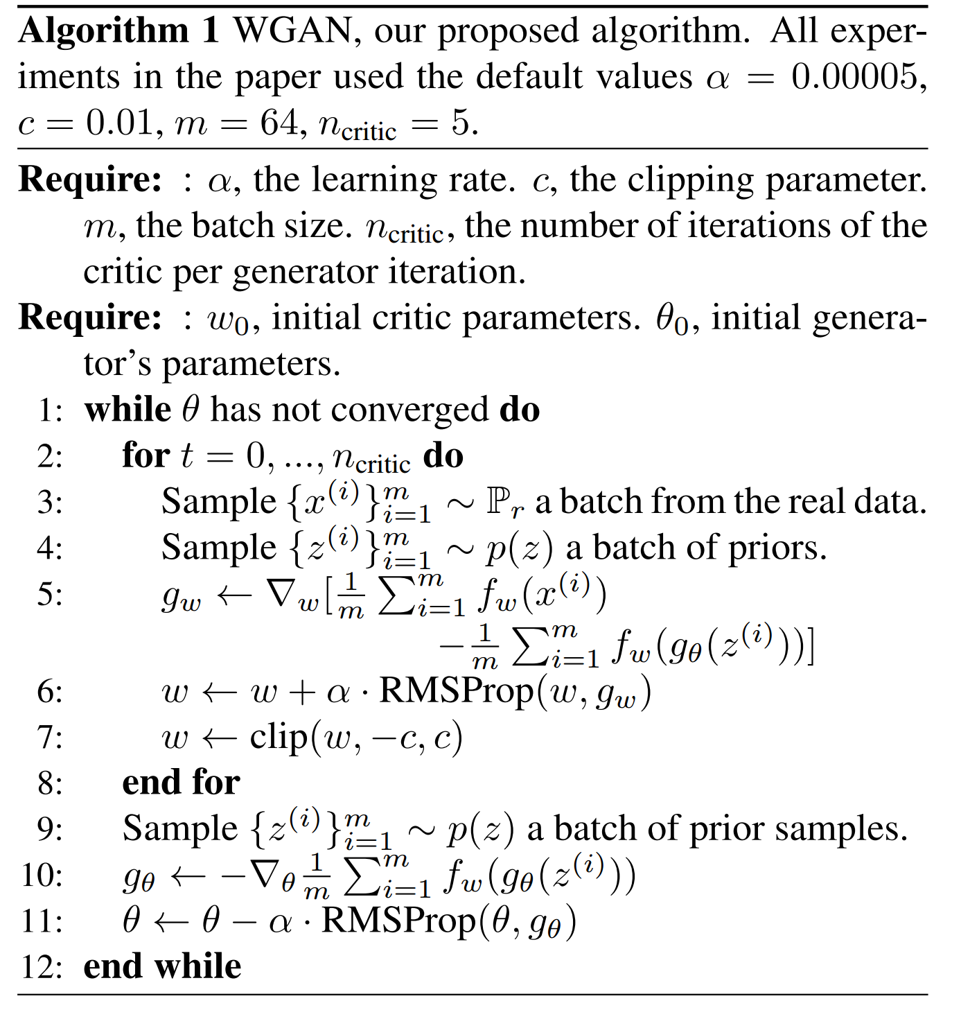
图 4. WGAN 算法
每更新 n 步判别器, 更新 1 步生成器. 判别器参数每次更新后都要裁剪到 [-c, c] 的范围内.
另外, WGAN 能够正常的把判别器训练到最优, 也可以避免 mode collapse 的问题. 这是因为 model collapse 问题来自于: 对于固定的判别器, 最优的生成器是判别器赋以最大值的那些点上的 delta 函数之和.
3. 实验结果
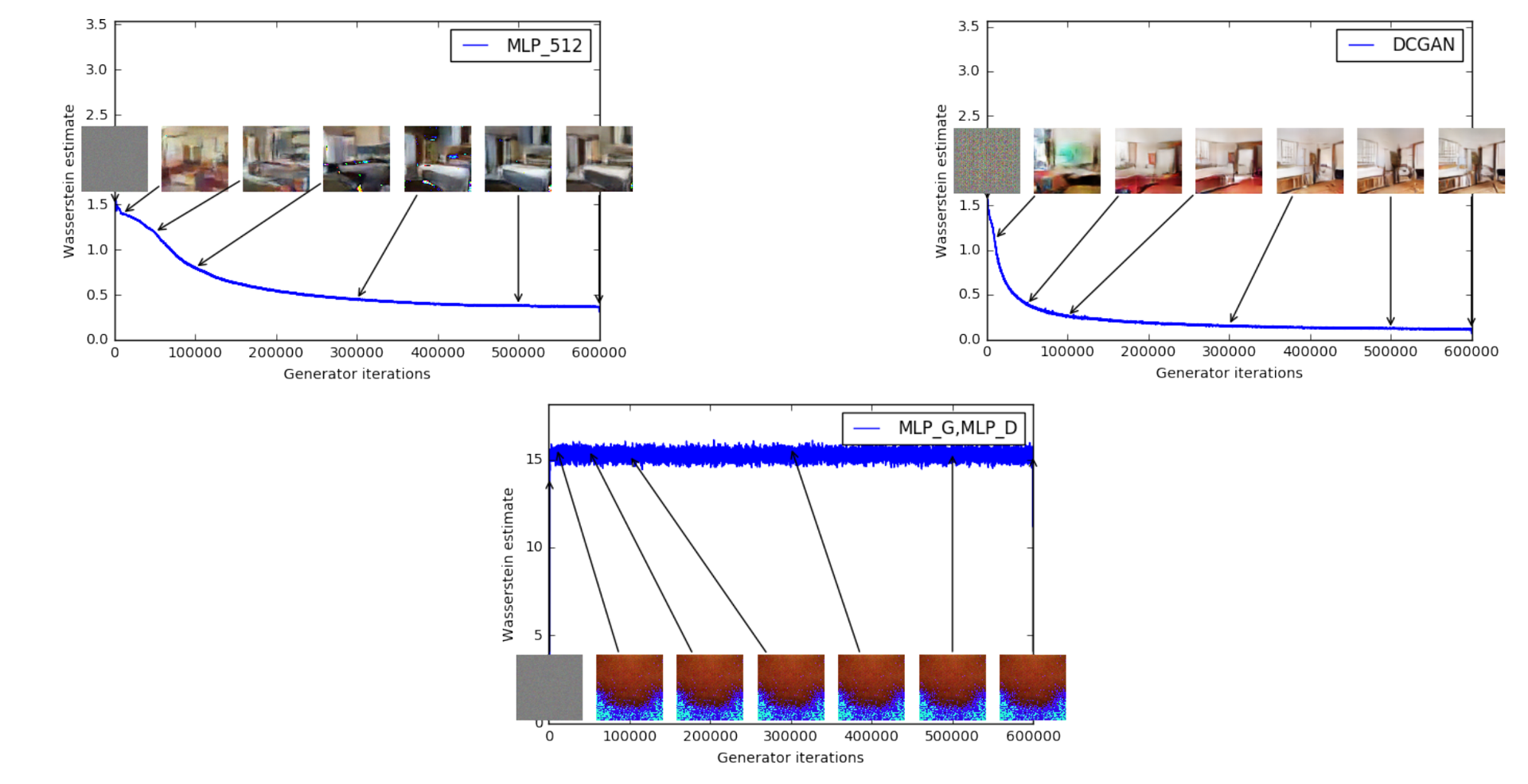
图 5. WGAN 损失函数的收敛情况
上图是用 WGAN 训练的损失函数的变化过程以及对应的生成的结果. 上面两幅图的判别器都用的DCGAN, 生成器分别用 MLP_512 和 DCGAN; 下面一幅图的生成器和判别器都用 MLP. 上面两幅图的结果来看, EM 损失都收敛了. 作者表示这可能是截止当时 GAN 的训练中首次实现损失函数的正常收敛.
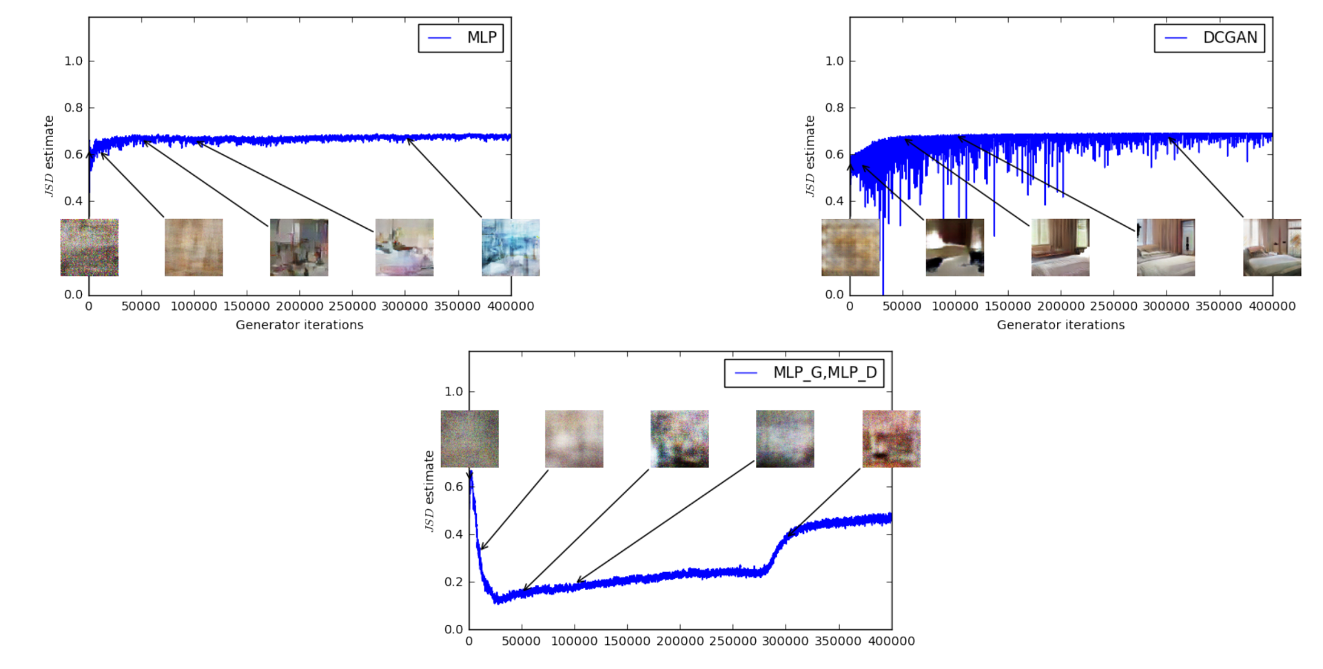
图 6. JSD 损失函数的收敛情况
与WGAN之相比, 上图使用JS距离来训练GAN, 其损失函数甚至都不降反升, 最终趋于log2=0.69附近, 这表明判别器的损失已经为0了, 而生成的样本有时是有意义的, 但有时又陷入 mode collapse.
另外, 本文指出了WGAN 的一个副作用, 即使用基于动量的优化方法(比如Adam)优化判别器时, 或者设置较大的学习率时, 训练过程会变得非常不稳定. 因此本文使用 RMSProp 来作为优化器训练判别器.
最后, 本文发现使用WGAN时, 对生成器的网络结构比较宽容.